 |
Often, we have available high-resolution (atomic) information for the subunits in an assembly, and low-resolution information for the assembly as a whole (a cryo-EM electron density map). A high-resolution model of the whole assembly can thus be constructed by simultaneously fitting the subunits into the density map. Fitting of a single protein into a density map is usually done by calculating the electron density of the protein followed by a search of the protein position in the cryo-EM map that maximizes the cross correlation of the two maps. Simultaneously fitting multiple proteins into a given map is significantly more difficult, since an incorrect fit of one protein will also prevent other proteins from being placed correctly.
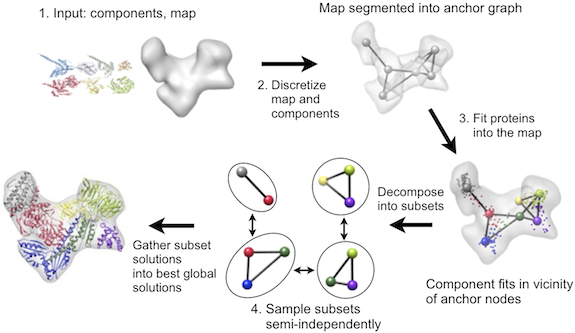
IMP contains a multifit module that can efficiently solve such multiple fitting problems for density map resolutions as low as 25Å, relying on a general inferential optimizer DOMINO. The fitting protocol is a multi-step procedure that proceeds via discretization of both the map and the proteins, local fitting of the proteins into the map, and an efficient combination of local fits into global solutions:
Currently, MultiFit is not distributed with IMP itself, and must be downloaded separately.
Here, we will demonstrate the use of multifit in building a model of the ARP2/3 complex using crystal structures of its seven constituent proteins (ARP2, ARP3, and ARC1-5) and a 20Å density map of the assembly. All input files for this procedure can be found in this zipfile.
The first step in using multifit is to create input files that guide the protocol. The first of these files, assembly.input, lists each of the subunits and the density map, complete with the names of the files from which the input structures and map will be read, and those to which outputs from later steps will be written. In this case, we also know the native structure of the assembly (PDB code 1tyq) and so we add the subunit structures in native conformation to this input file (rightmost column); multifit will use them to assess its accuracy. Normally, of course, the real native structure is not known, in which case this column in the input file is left blank. The second file, multifit.par, specifies various optimization parameters, and is described in more detail on the multifit website.
The second step is to determine a reduced representation for both the density map and the subunits, using the Gaussian Mixture Model. This task can be achieved by typing, in the directory containing assembly.input (the syntax for running Python scripts may vary depending on where the files are installed):
/opt/multifit/utils/run_anchor_points_detection.py assembly.input 700
This run determines a reduced representation of the EM map that best reproduces the configuration of all voxels with density above 700, and a similar reduced representation of each subunit as a set of 3D Gaussian functions. The number of Gaussians is specified in assembly.input for each subunit. It should be at least 3 (the minimum required for fitting) and each Gaussian should cover approximately the same number of residues (for example, if you choose 50 residues per Gaussian, a 170-residue protein should use 3 Gaussians and a 260-residue protein should use 5 Gaussians). Each such reduced map representation can also be thought of as an anchor point graph, where each anchor point corresponds to the center of a 3D Gaussian, and the edges in the graph correspond to the connectivity between regions of the map or protein. These reduced representations are written out as PDB files containing fake Cα atoms, where each Cα corresponds to a single anchor point.
The third step is to fit each protein in the vicinity of the EM map’s anchor points. This task is achieved by running:
/opt/multifit/utils/run_protein_fitting.py assembly.input multifit.par
The output is a set of candidate fits, where the subunit is rigidly rotated and translated to fit into the density map. Each fit is written as a PDB file in the ‘fits’ subdirectory. The fitting procedure is performed by either aligning a reduced representation of a protein to a reduced representation of the density map or by fitting the protein principal components to the principal components of a segmented region of the map.
Finally, the fits are scored and then combined into a set of the best-scoring global configurations:
/opt/multifit/utils/run_all_scores.py assembly.input > scores.log
/opt/multifit/utils/run_multifit.py assembly.input assembly.jt assembly_configurations.output data/models/1tyq.fitted.pdb > multifit.log
The scoring function used to assess each fit includes the quality-of-fit of each subunit into the map, the protrusion of each subunit out of the map envelope, and the shape complementarity between pairs of neighboring subunits. The optimization avoids exhaustive enumeration of all possible mappings of subunits to anchor points by means of a branch-and-bound algorithm combined with the DOMINO divide-and-conquer message-passing optimizer using a discrete sampling space.
The final output from multifit is a file assembly_configurations.output that lists the best global solutions, ranked by their score, an excerpt of which is shown below:
ARP3,0|ARP2,14|ARC1,3|ARC2,24|ARC3,19|ARC4,11|ARC5,13|(17.5593729019)(rmsd:29.2637996674)(conf.0.pdb)
ARP3,5|ARP2,13|ARC1,9|ARC2,24|ARC3,19|ARC4,4|ARC5,13|(18.3258602619)(rmsd:11.997220993)(conf.1.pdb)
For each global solution, multifit lists the indices of the local fits for each subunit and the score. Each solution is also written out as a multi-chain PDB file of the assembly. In addition, because we also provided the native structure (1tyq.fitted.pdb), the RMSD between the native conformation and each solution is listed. In this case, the RMSD measure indicates that multifit has correctly determined the architecture of the assembly, placing each subunit in the approximately correct part of the map. However, the protein-protein interfaces are clearly not accurate at the atomic level. These models could thus be refined with a combination of pairwise computational docking and local sampling, ideally supported by additional experimental data, such as chemical cross-linking, various kinds of footprinting, and X-ray crystallography of binary subunit complexes.